Background
We performed a series of simulation studies to test some of the estimation properties of a subset of the ROC core-computation functions. With time we will provide similar information about all functions. We performed our simulations in the Matlab computing environment on a Linux cluster. Other simulations have shown that calling the functions from different operating systems (e.g., Windows, OS X) or environments (R or command line) appears to affect results in a negligible way (e.g., difference in AUC ~ .000000001). We have only recently begun providing support for Matlab. Our simulation studies therefore had three purposes: to study in detail the behavior of these functions; to verify that the behavior of the library’s interface under Matlab is consistent in “look and feel” with native matlab functions; and, to verify that the results of those simulation studies are consistent with the results obtained from the library functions under other computing environments.
The purpose of the simulations is to explore and appraise how well our functions estimate indices of interest when applied to random samples from a population whose properties are known. We chose a population following the so-called contaminated binormal model of Dorfman et al. because it provides curves that are convex, which is desirable, but that do not follow the mathematical form of the models tested here therefore providing a degree of model misspecification. Four different underlying parameter sets of the underlying data model (values of the a parameter of the conventional binormal model, and the value of the alpha parameter of the contaminated binormal model) were considered. In practice this means that we have studied the behavior of the functions as we varied the population ROC area under the curve and shape. For each of these, six different dataset sizes (ranging from 25 actually-positive and 25 actually-negative cases, i.e., a small balanced dataset, up to 20 actually-positive and 180 actually-negative cases, i.e., a larger but unbalanced dataset) were considered.
Three ROC models were tested: the conventional binormal model (CvBM), the proper binormal model (PBM) and the non-parametric model (empirical ROC curve). Please note that although some of the mean results differ significantly from the corresponding true values, many of those differences are small.
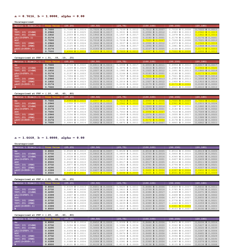
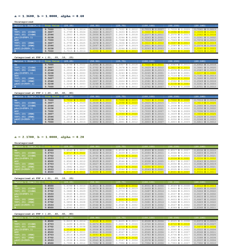
For a given parameter set and dataset size, observations were generated using a normally distributed random-number generator, and then “categorized” into three different categorization states: uncategorized (the data were left unchanged — so-called quasi-continuous data); categorized with category boundaries at FPF equal to .01, .05, .10, and .25 (ordinal-categorical data with operating points for medium/large specificity values as usually observed in mammography, for example); and categorized with boundaries at FPF equal to .20, .40, .60, and .80 (ordinal-categorical, but uniformly distributed on the specificity axis). For each study condition (parameter set, dataset size, categorization state), 10,000 such datasets were generated, and the values of nine performance metrics:
Area under the ROC curve (indicated in the tables with Az for CvBM, AUC for PBM and W for non-parametric — from the Wilcoxon statistic)
TPF at FPF (only for CvBM and PBM) for FPF values equal to .05 and .1
Partial area under the curve (indicated with pAz for CvBM and pAUC for PBM) computed between FPF=0 and FPF = .1
The means plus or minus 1.96 standard errors (giving 95% confidence intervals under the normality assumption) across these 10,000 datasets are reported in the tables below for each of the study conditions. Conditions for which the true value of the performance metric lies within this confidence interval are indicated by yellow highlighting.
Simulation Study Results
You can also download a PDF version here.